This is a tool for code fault analysis. I built it to automate the most boring part of my debugging process.
The package automates test setup and logging and visualizes function exit states in a way that simplifies identification of root causes of software defects. Fuzzing is implemented by random generation of input parameters as shown in a demo below. Finally, even though there was no goal to make this tool as another unit testing package, one can use it as such, as this tool should potentially assure 100% code coverage with minimal effort.
The package tests all possible combinations of input parameters and produces statistics and visuals. If you have some specific requirements, you can simply build a wrapper function that catches output you are interested in and generates an error if a required condition is not met. Then submit your wrapper function for testing. You can even compare current output values against values recorded in a log during a ‘reference’ test run, effectively making a comprehensive unit test.
The package can be installed from here: https://github.com/cloudcell/fuzztest/.
Below is a presentation of a built-in demo. You can run it using `demo(fuzzdemo)`.
I will be grateful for your comments and suggestions.
> demo(fuzzdemo)
    r <- list()
    r$x <- c(0)
    r$y <- c(0)
    r$option <- c("a", "b", "c")
    r$suboption <- c("a", "b", "c","d")

    generate.argset(arg_register = r, display_progress=TRUE)
    apply.argset(FUN="fuzzdemofunc")
    test_summary()
    plot_tests()
    plot_tests(fail = F)
    plot_tests(pass = F)
===LOG OMITTED===
Fuzztest: Argument-Option Combination Results
===================================================
ARG~OPT Arg Name PASS FAIL FAIL%
---------------------------------------------------
1 ~ 1 x 5 7 58.3
2 ~ 1 y 5 7 58.3
3 ~ 1 option 4 0 0.0
3 ~ 2 option 1 3 75.0
3 ~ 3 option 0 4 100.0
4 ~ 1 suboption 2 1 33.3
4 ~ 2 suboption 1 2 66.7
4 ~ 3 suboption 1 2 66.7
4 ~ 4 suboption 1 2 66.7
===================================================
Fuzztest: Summary
========================================================================
Arg Name Failure Rate Contribution, % (Max - Min)
------------------------------------------------------------------------
x 0.0 ' '
y 0.0 ' '
option 100.0 '**************************************************'
suboption 33.3 '***************** '
========================================================================
The summary shows that the argument 'option' explains the most
variability in the outcome. So let's concentrate on the arg. 'option.'
The detailed statistics table shows that most failures occur when
value #3 is selected within the argument 'option'. At the same time,
a test log (omitted here) shows that the types of errors are mixed.
For now, however, let's assume that fixing the bugs related to
control flow is more important.
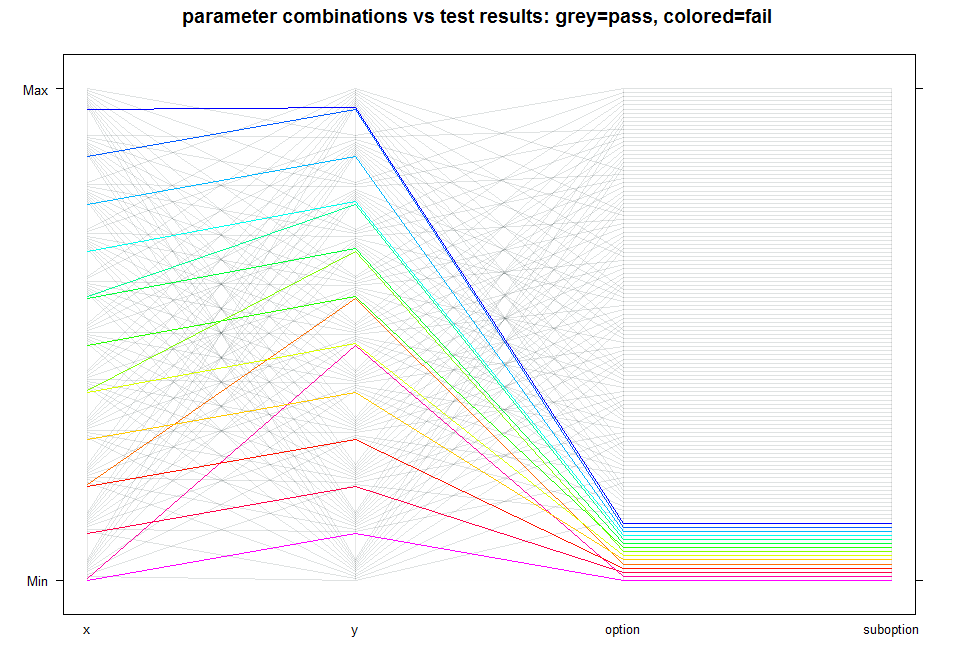
The following three graphs will demonstrate how the data above
can be represented visually. Notice that some lines are grouped
when they intersect vertical axes. The groups correspond to specific
options and are ordered from the bottom of the chart to the top:
i.e. the fist grouping of lines at axis 'suboption' (at the bottom)
corresponds to value 'a', the next one up is suboption 'b', and so on.
In case an argument has only one value in the test, the whole
group of lines will be evenly spread from the bottom to the top of
the chart, as is the case for arguments 'x' and 'y'.
* All test cases:
 One can also selectively display only passing or failing tests
as will be shown next.
* Only 'passing' test cases:
One can also selectively display only passing or failing tests
as will be shown next.
* Only 'passing' test cases:
 * Only 'failing' test cases:
 Let's assume all the control flow related bugs discussed above
are fixed now. To make this assumption to "work" during testing
we will simply choose a combination of options that will not
cause the demo function to produce 'fail' states shown above.
Such a combination could be {x=0, y=0, option='a', suboption='a'}.
Now we will concentrate on the numeric part of the test.
There are two main testing approaches:
1. Create an evenly spaced sequence of values for each parameter
(x and y) from lowest to highest and let the argument set generator
combine and test these values. This approach has an advantage
for more intuitive visualization as sequences of values
for testing will be aligned with the vertical axis. For example,
if we create a test sequence [-10;+10] for argument 'x',
visualized test results will list those from 'Min' to 'Max'.
So finding simple linear dependencies that cause errors will
be easier as it will be easier than when using a random set
of values (below).
2. Generate random parameters for selected arguments and let the test
framework test all possible parameter combinations.
The First Approach: Ordered Test Sequences
Let's assume all the control flow related bugs discussed above
are fixed now. To make this assumption to "work" during testing
we will simply choose a combination of options that will not
cause the demo function to produce 'fail' states shown above.
Such a combination could be {x=0, y=0, option='a', suboption='a'}.
Now we will concentrate on the numeric part of the test.
There are two main testing approaches:
1. Create an evenly spaced sequence of values for each parameter
(x and y) from lowest to highest and let the argument set generator
combine and test these values. This approach has an advantage
for more intuitive visualization as sequences of values
for testing will be aligned with the vertical axis. For example,
if we create a test sequence [-10;+10] for argument 'x',
visualized test results will list those from 'Min' to 'Max'.
So finding simple linear dependencies that cause errors will
be easier as it will be easier than when using a random set
of values (below).
2. Generate random parameters for selected arguments and let the test
framework test all possible parameter combinations.
The First Approach: Ordered Test Sequences
    r <- list()
    r$x <- c(seq(from=-5, to=5, length.out = 11))
    r$y <- c(seq(from=-5, to=5, length.out = 11))
    r$option <- c("a")
    r$suboption <- c("a")

    generate.argset(arg_register = r, display_progress=TRUE)
    apply.argset(FUN="fuzzdemofunc")
    test_summary()
    plot_tests()
===LOG OMITTED===

Fuzztest: Argument-Option Combination Results
===================================================
   ARG~OPT     Arg Name     PASS    FAIL    FAIL%
---------------------------------------------------
   1 ~    1    x               9       2     18.2
   1 ~    2    x              10       1     9.09
   1 ~    3    x               9       2     18.2
   1 ~    4    x              10       1     9.09
   1 ~    5    x               9       2     18.2
   1 ~    6    x              10       1     9.09
   1 ~    7    x               9       2     18.2
   1 ~    8    x              10       1     9.09
   1 ~    9    x              10       1     9.09
   1 ~   10    x              10       1     9.09
   1 ~   11    x              10       1     9.09
   2 ~    1    y              11       0      0.0
   2 ~    2    y              10       1     9.09
   2 ~    3    y              10       1     9.09
   2 ~    4    y              10       1     9.09
   2 ~    5    y              10       1     9.09
   2 ~    6    y               9       2     18.2
   2 ~    7    y               9       2     18.2
   2 ~    8    y               9       2     18.2
   2 ~    9    y               9       2     18.2
   2 ~   10    y              10       1     9.09
   2 ~   11    y               9       2     18.2
   3 ~    1    option        106      15     12.4
   4 ~    1    suboption     106      15     12.4
===================================================

Fuzztest: Summary
========================================================================
  Arg Name            Failure Rate Contribution, % (Max - Min)
------------------------------------------------------------------------
          x   9.09  '*****                                             '
          y   18.2  '*********                                         '
     option    0.0  '                                                  '
  suboption    0.0  '                                                  '
========================================================================

The test summary shows that argument 'y' contributes to
failure the most.

What about the chart?


Now one can clearly see two linear relationships between
'x' and 'y'. These correspond to 'numeric bugs' #1NC and #4NC
(Please, see details in the file 'include_fuzzdemofunc.R')

Let's assume the previously discovered bugs have been fixed.
So we will again choose a different combination of input parameters
for arguments 'option' and 'suboption' for the next test.


The Second Approach: Random Test Sequences

It makes no sense testing options randomly as all those
combinations of values will be tested anyway. So the test
will be conducted for numeric arguments only.

This test has 900 cases and might take a couple of minutes,
so you have time to pour yourself a cup of coffee: (_)]...
Now one can clearly see two linear relationships between
'x' and 'y'. These correspond to 'numeric bugs' #1NC and #4NC
(Please, see details in the file 'include_fuzzdemofunc.R')
Let's assume the previously discovered bugs have been fixed.
So we will again choose a different combination of input parameters
for arguments 'option' and 'suboption' for the next test.
The Second Approach: Random Test Sequences
It makes no sense testing options randomly as all those
combinations of values will be tested anyway. So the test
will be conducted for numeric arguments only.
This test has 900 cases and might take a couple of minutes,
so you have time to pour yourself a cup of coffee: (_)]...
    set.seed(0)
    r <- list()
    r$x <- runif(15, min=-10, max=10)
    r$y <- runif(15, min=-10, max=10)
    r$option <- c("b")
    r$suboption <- c("a","b","c","d")

    generate.argset(arg_register = r, display_progress=TRUE)
    apply.argset(FUN="fuzzdemofunc")
    test_summary()
    plot_tests()
===LOG OMITTED===

Fuzztest: Argument-Option Combination Results
===================================================
   ARG~OPT     Arg Name     PASS    FAIL    FAIL%
---------------------------------------------------
   1 ~    1    x              35      25     41.7
   1 ~    2    x              35      25     41.7
   1 ~    3    x              35      25     41.7
   1 ~    4    x              35      25     41.7
   1 ~    5    x              35      25     41.7
   1 ~    6    x              35      25     41.7
   1 ~    7    x              35      25     41.7
   1 ~    8    x              35      25     41.7
   1 ~    9    x              35      25     41.7
   1 ~   10    x              35      25     41.7
   1 ~   11    x              35      25     41.7
   1 ~   12    x              35      25     41.7
   1 ~   13    x              35      25     41.7
   1 ~   14    x              35      25     41.7
   1 ~   15    x              35      25     41.7
   2 ~    1    y              45      15     25.0
   2 ~    2    y              30      30     50.0
   2 ~    3    y              30      30     50.0
   2 ~    4    y              45      15     25.0
   2 ~    5    y              30      30     50.0
   2 ~    6    y              45      15     25.0
   2 ~    7    y              45      15     25.0
   2 ~    8    y              30      30     50.0
   2 ~    9    y              30      30     50.0
   2 ~   10    y              30      30     50.0
   2 ~   11    y              30      30     50.0
   2 ~   12    y              30      30     50.0
   2 ~   13    y              30      30     50.0
   2 ~   14    y              30      30     50.0
   2 ~   15    y              45      15     25.0
   3 ~    1    option        525     375     41.7
   4 ~    1    suboption     225       0      0.0
   4 ~    2    suboption     195      30     13.3
   4 ~    3    suboption       0     225    100.0
   4 ~    4    suboption     105     120     53.3
===================================================

Fuzztest: Summary
========================================================================
  Arg Name            Failure Rate Contribution, % (Max - Min)
------------------------------------------------------------------------
          x    0.0  '                                                  '
          y   25.0  '************                                      '
     option    0.0  '                                                  '
  suboption  100.0  '**************************************************'
========================================================================

The test table shows that suboption #3 ('c') is always failing.

Let's see if the visual approach provides a better perspective.


This graph has a confusing order of axes at this point.
An axis that has only one option should either be hidden or placed
at an edge of the chart so relations with other parameters could
be visible. To reorder axes, for simplicity, we will quickly create
a smaller test with a different sequence of arguments, which will
change the sequence of axes.
    set.seed(0)
    r <- list()
    r$x <- runif(5, min=-10, max=10)
    r$y <- runif(5, min=-10, max=10)
    r$suboption <- c("a","b","c","d")
    r$option <- c("b")

    generate.argset(arg_register = r, display_progress=TRUE)
    apply.argset(FUN="fuzzdemofunc")
    test_summary()
    plot_tests()
===LOG OMITTED===

Fuzztest: Argument-Option Combination Results
===================================================
   ARG~OPT     Arg Name     PASS    FAIL    FAIL%
---------------------------------------------------
   1 ~    1    x              12       8     40.0
   1 ~    2    x              12       8     40.0
   1 ~    3    x              12       8     40.0
   1 ~    4    x              12       8     40.0
   1 ~    5    x              12       8     40.0
   2 ~    1    y              10      10     50.0
   2 ~    2    y              15       5     25.0
   2 ~    3    y              15       5     25.0
   2 ~    4    y              10      10     50.0
   2 ~    5    y              10      10     50.0
   3 ~    1    suboption      25       0      0.0
   3 ~    2    suboption      15      10     40.0
   3 ~    3    suboption       0      25    100.0
   3 ~    4    suboption      20       5     20.0
   4 ~    1    option         60      40     40.0
===================================================

Fuzztest: Summary
========================================================================
  Arg Name            Failure Rate Contribution, % (Max - Min)
------------------------------------------------------------------------
          x    0.0  '                                                  '
          y   25.0  '************                                      '
  suboption  100.0  '**************************************************'
     option    0.0  '                                                  '
========================================================================


The textual test summary shows the same pattern as in the previous
test. Also, a reduced set of test cases produced a more transparent
representation of test results without losing important details.

There are many ways to proceed from here:
* if some 'error' states are valid, one can exclude them from tests
  using the 'subset' argument of apply.argset().
* if bugs are trivial, one can eliminate them one by one.
* if faults are intractable, one can start with narrowing down the
  range of input parameters and further analyze function behavior.

-------------
 End of Demo
-------------
The textual test summary shows the same pattern as in the previous
test. Also, a reduced set of test cases produced a more transparent
representation of test results without losing important details.
There are many ways to proceed from here:
* if some 'error' states are valid, one can exclude them from tests
using the 'subset' argument of apply.argset().
* if bugs are trivial, one can eliminate them one by one.
* if faults are intractable, one can start with narrowing down the
range of input parameters and further analyze function behavior.
-------------
End of Demo
-------------
The following is the test function used in the demo
#' Generates errors for several combinations of input parameters to test the
#' existing and emerging functionality of the package
#'
#' Whenever options lead the control flow within a function to a 'demo bug',
#' the function stops and the test framework records a 'FAIL' result.
#' Upon a successful completion, the function returns a numeric value into the
#' environment from which the function was called.
#'
#' @param x: any numeric scalar value (non-vector)
#' @param y: any numeric scalar value (non-vector)
#' @param option any character value from "a", "b", "c"
#' @param suboption any character value from "a", "b", "c", "d"
#'
#' @author cloudcell
#'
#' @export
fuzzdemofunc <- function(x, y, option, suboption)
{
    tmp1 <- 0
    switch(option,
           "a"={
               switch(suboption,
                      "a"={                                    },
                      "b"={                                    },
                      "c"={ if(x + y <0) stop("demo bug #1CF (control flow)") },
                      "d"={                                    },
                      { stop("Wrong suboption (valid 'FAIL')") }
               )
               if(abs(x-y+1)<0.01) stop("demo bug #1NC (numeric calc.)")
           },
           "b"={
               x <- 1
               switch(suboption,
                      "a"={ x <- x*1.5                         },
                      "b"={ x <- y                             },
                      "c"={ y <- 1 }, "d"={ if(x>y) stop("demo bug #2CF (control flow)") },
                      { stop("Wrong suboption (valid 'FAIL')") }
               )
               if(abs(x %% 5 - y)<0.01) stop("demo bug #2NC (numeric calc.)")
           },
           "c"={
               switch(suboption,
                      "a"={ stop("demo bug #3CF (control flow)") },
                      "b"={                                    },
                      "c"={                                    },
                      "d"={  rm(tmp1)                          },
                      { stop("Wrong suboption (valid 'FAIL')") }
               )
               if(abs(x %/% 5 - y)<0.01) stop("demo bug #3NC  (numeric calc.)")
           },
           { stop("Wrong option (valid 'FAIL')") }
    )

    if(!exists("tmp1")) stop("demo bug #4CF (control flow)")

    result <- x - y*2 + 5

    if(abs(result)<0.01) stop("demo bug #4NC  (numeric calc.)")

    result
}


